Retrieval
Default settings
The default retrieval setting of HyperGas is matched filter with watermask defined by OSM and ESA WorldCover.
>>> hyp.retrieve(species='ch4')
hypergas.unit_spectrum - INFO: Read atm file: atmosphere_midlatitudewinter.dat
hypergas.unit_spectrum - INFO: Convolving rads (2110~2450 nm) ...
hypergas.unit_spectrum - INFO: Convolving rads (Done)
hypergas.landmask - INFO: Creating land mask using OSM data
hypergas.landmask - INFO: Creating land mask using OSM data (Done)
hypergas.retrieve - INFO: Applying matched filter ...
Retrieval output:
>>> print(hyp.scene['ch4'])
<xarray.DataArray 'ch4' (bands: 1, y: 1280, x: 1242)> Size: 6MB
array([[[  19.328018 ,   -7.9269505,   86.22249  , ...,  -67.75732  ,
        -104.04307  ,  -50.041225 ],
        [ -30.324438 ,   50.841778 ,  -20.87884  , ...,   35.689144 ,
        -63.426575 ,  -19.803162 ],
        [ -11.326984 ,   35.69191  ,    3.8998451, ...,    8.005404 ,
        -51.085037 ,  -90.70705  ],
        ...,
        [ 616.1246   ,   59.302395 ,  143.64334  , ..., -283.39716  ,
        285.37698  ,  533.53125  ],
        [-136.13683  ,  135.83197  ,   32.05849  , ...,  -80.42325  ,
        394.68613  ,  301.15356  ],
        [ -82.05242  ,  182.5513   ,    6.4179454, ...,   87.19298  ,
        346.68774  ,  339.0367   ]]], dtype=float32)
Dimensions without coordinates: bands, y, x
Attributes: (12/22)
    long_name:            methane_enhancement
    units:                ppb
    name:                 ch4
    file_type:            ['emit_l1b_rad']
    standard_name:        methane_enhancement
    nc_group:             None
    ...                   ...
    _satpy_id:            DataID(name='ch4', modifiers=())
    ancillary_variables:  []
    sza:                  30.461334228515625
    vza:                  9.43835163116455
    description:          methane enhancement derived by the 2110~2450 nm window
    matched_filter:       normal matched filter
HyperGas provides different options for retrieval algorithm and watermask/cluster:
- algorithms
matched filter
lognormal matched filter
cluster-tuned matched filter
- watermask/cluster
OSM and ESA WorldCover
the Global Self-consistent, Hierarchical, High-resolution Geography database (GSHHG)
the Natural Earth dataset
k-means clustering
The default wavelength windows for each trace gas are defined in <HyperGas_dir>/hypergas/config.yaml.
See Developer’s Guide for more information.
Users can test wavelength ranges temporarily by modifying the wvl_intervals parameter,
which can be a list or multi-list.
>>> hyp.retrieve(wvl_intervals=[1300, 2500], species='ch4')
>>> hyp.retrieve(wvl_intervals=[[1600, 1750], [2110, 2450]], species='ch4')
Algorithms
Matched filter
The matched filter (Thompson et al. 2015, Foote et al. 2021) treats the background spectral signature as a Gaussian distribution with a mean vector \(\mu\) and a covariance matrix \(\Sigma\). The radiance spectrum (\(L\)) can be represented by two hypotheses: H0, which assumes the absence of plume, and H1, where the plume is present.
Here, \(t\) represents the target signature, which is the product of two components: the background radiance (\(\mu\)) and the negative gas absorption coefficient (\(k\)). To calculate \(k\), we employ a forward model and convolve it with the imager’s central wavelength and full width at half maxima (FWHM). The scale factor \(\alpha\) is derived from the first-order Taylor expansion of Beer-Lambert’s law. The maximum likelihood estimate of \(\alpha\) is:
Lognormal matched filter
One limitation of the matched filter is the linear approximation, which could lead to underestimation of big emitting plumes. Thus, HyperGas provides the lognormal matched filter method (Schaum et al. 2021, Pei. et al. 2023), which applies logarithms to both sides of the Beer-Lambert equation:
Here, the new \(\tilde{\mu}\) is the mean log background radiance and \(\tilde{\Sigma}\) is the covariance matrix of the log background radiance, , and \(\tilde{L}\) is the log radiance spectrum.
Users can swtich to lognormal matched filter by passing rad_dist='lognormal':
>>> hyp.retrieve(species='ch4', rad_dist='lognormal')
Cluster-tuned matched filter
Studies suggest that applying the matched filter to clustered pixels can reduce background noise such as the albedo effect caused by roads and roofs. HyperGas supports reducing the dimension of data space by principal component analysis (PCA) and then classifying them into clusters by the k-means algorithm. Users need to take care of the results because the cluster-tuned matched filter can sometimes make results noisier.
>>> hyp.retrieve(species='ch4', cluster=True)
Landmask/Cluster
Due to the high spatial resolution of HSIs, HyperGas classifies pixels by integrating data from both OpenStreetMap (OSM)
and ESA WorldCover databases.
There are other three options (GSHHG, Natural Earth, and K-means) for the MatchedFilter.
Users can adjust the watermask/cluster by setting the cluster and land_mask_source kwargs:
>>> hyp.retrieve(rad_dist='normal', cluster=False, land_mask_source='OSM')  # default: OSM land/water mask
>>> hyp.retrieve(rad_dist='normal', cluster=False, land_mask_source='GSHHS')    # GSHHG land/water mask
>>> hyp.retrieve(rad_dist='normal', cluster=True)  # kmeans clusters
Once the cluster is turned on, the land_mask_source would not be applied.
Users can also combine different algorithms and masks:
>>> hyp.retrieve(rad_dist='lognormal', land_mask_source='OSM') # OSM land/water mask with lognormal matched filter
Databases
OSM and ESA WorldCover
The processed data has been handled by the Alaska Satellite Facility. The geographic coverage is distributed as follows: ESA WorldCover data primarily encompasses Canada, Alaska, and Russia, while OpenStreetMap data covers the remaining global regions. These datasets were combined to create a global dataset. The implemented water mask effectively identifies both coastal waters and major inland water bodies. For regions beyond 85°S and 85°N, we apply a simplified classification: all areas north of 85°N are classified as water, while all areas south of 85°S are designated as non-water.
GSHHG and Natural Earth
HyperGas also supports two other datasets available through the cartopy feature interface: GSHHG and the 10-m Natural Earth dataset.
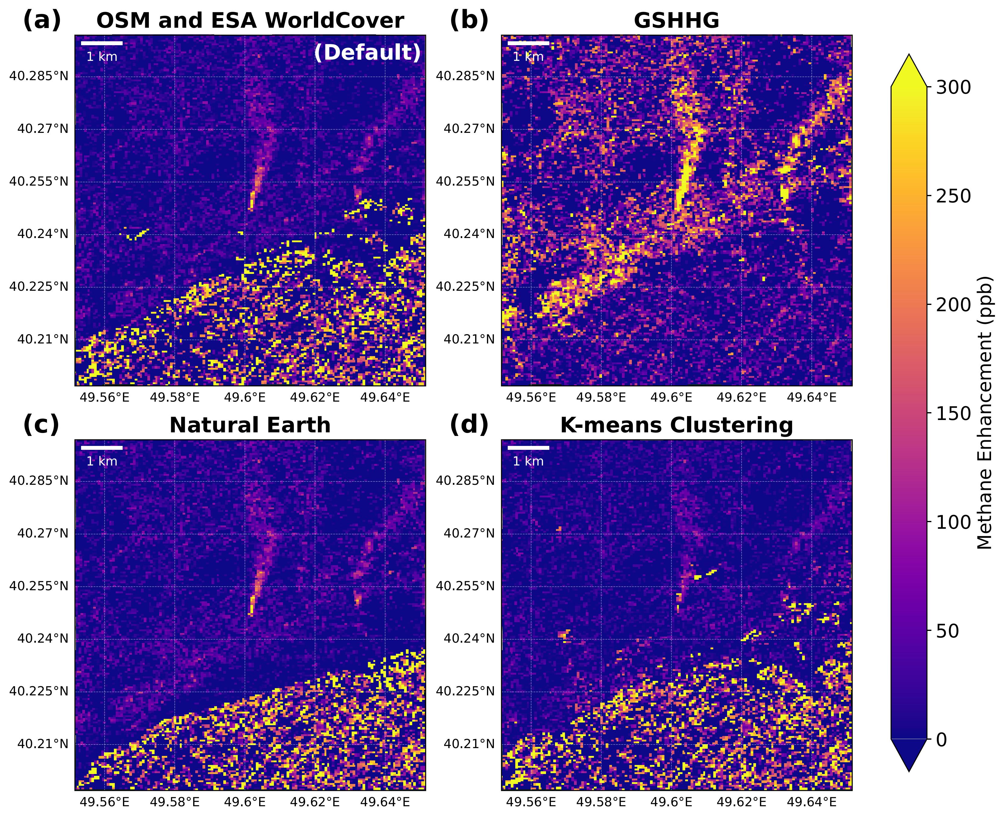
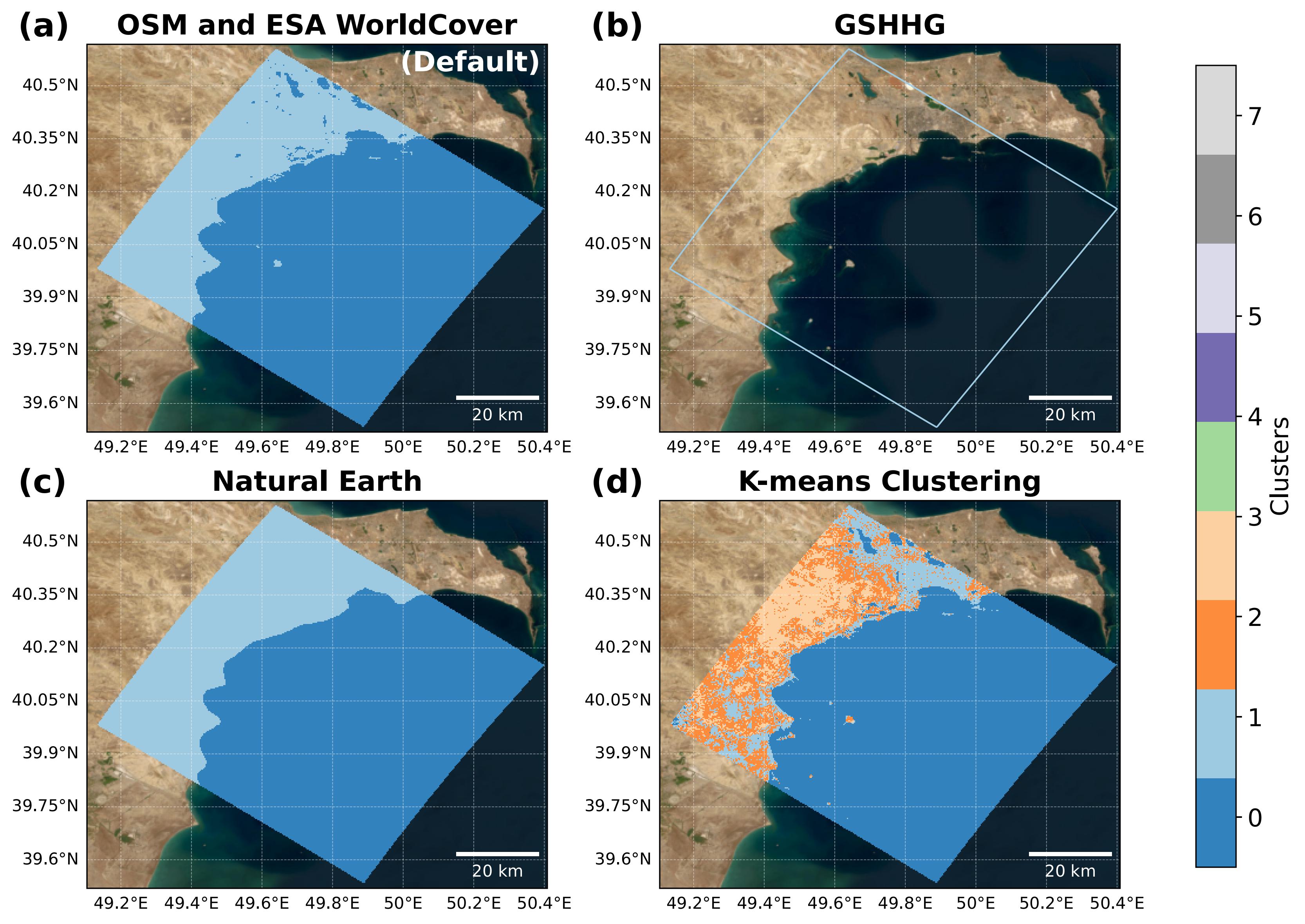
Comparisons
The figure below compares different water masks around the Caspian Sea. The OSM and ESA WorldCover datasets effectively differentiate between land and water, whereas the GSHHG dataset misclassifies some sea areas as land, and the Natural Earth dataset omits inland water bodies.
Here are the effects of different masks on methane retrieval: The results based on the GSHHG dataset tend to overestimate methane enhancement due to the mixture of land and water pixels. The results using the Natural Earth, OSM, and ESA WorldCover datasets are similar, whereas the k-means method produces a noisier image.