Plume APP
The Plume APP, built with Streamlit, offers two primary functions:
Adding markers for plume sources
Calculating emission rates using plume masks
Deploy
The Plume APP can be deployed on both local and remote machines.
Local
cd <HyperGas_dir>/app
streamlit run About.py
By default, the browser will automatically open the app. If it does not, manually open the browser and enter the local URL displayed in the terminal.
Remote
cd <HyperGas_dir>/app
streamlit run About.py --server.headless true --server.port 8501
For remote machines or servers, you can run the app on the server as above and access it via SSH:
ssh -N -L localhost:8501:localhost:8501 <username>@<server_ip>
Afterward, open your browser and navigate to http://localhost:8501/ to access the app.
Note
If port 8501 is already in use, you can change Streamlit’s default port to avoid conflicts.
Running the application in the background allows for easy access at any time. Tools like tmux, , which allow for multiple terminal panels and persistent sessions, are highly recommended for enhanced workflow.
Usage
1) Plume Marker
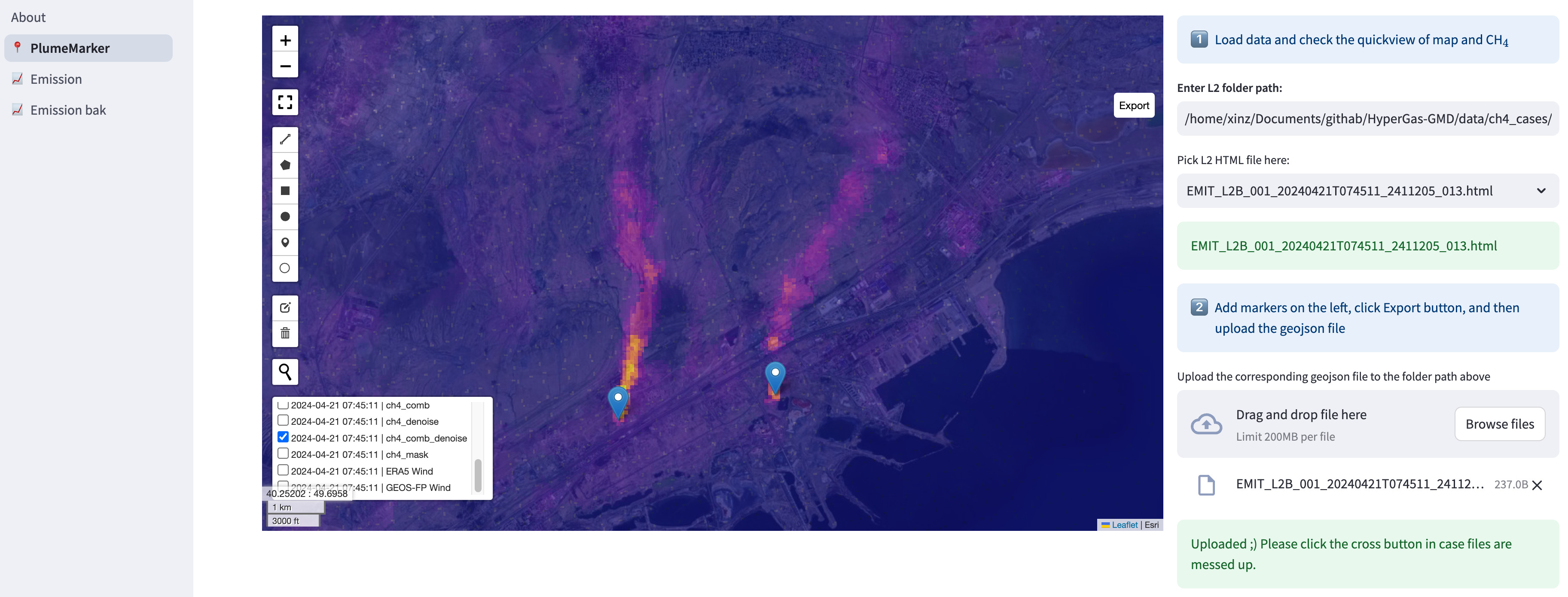
The PlumeMarker page includes a main preview window and two side panels.
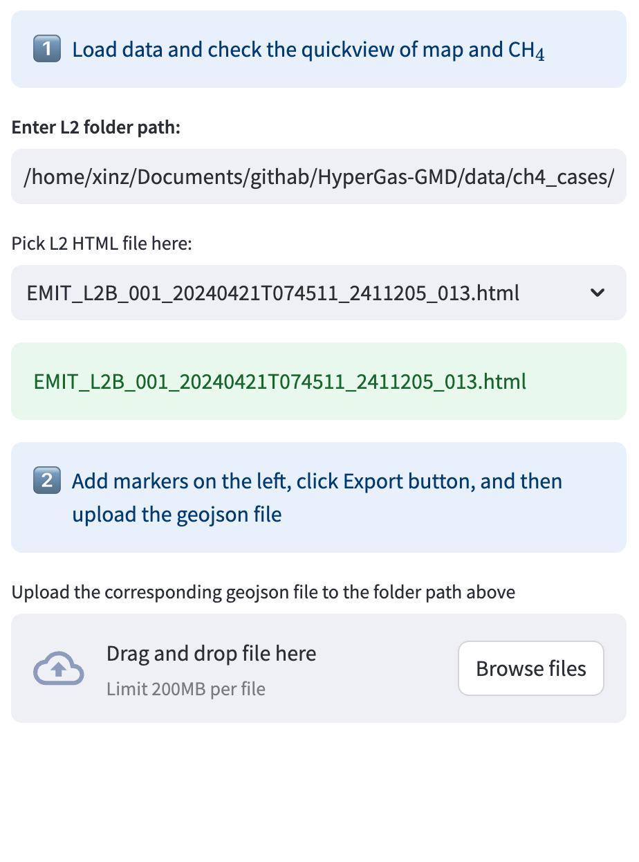
After entering the path to the L2 folder, the preview displays content identical to the HTML file generated by l2b_plot.py.
Users can then use the “Draw a marker” tool to identify multiple sources on the map. Once all hotspots have been defined, click the Export button in the top-right corner to generate a GeoJSON file.
Finally, users can click the “Browse files” button to either move the file locally or upload it remotely to the same directory as the L2 data.
Warning
The geojson files are essential for the next “Emission” step.
A green notification bar confirms the successful upload of the GeoJSON file. Click the “X” button to clear the cache. If the same path is used later, a warning will be shown.
2) Emission
The Emission page includes a primary preview window and three panels:
Load data
Create plume mask
Estimate emission rates
Note
These steps can also be automated using l3_process.py (see L2 –> L3/L4).
Load data
After verifying the folder path, the preview window will display the L2 or plume HTML file (if available). If the “I only want to check plume HTML files” toggle is enabled, only existing plume HTMLs will be shown.
Create plume mask
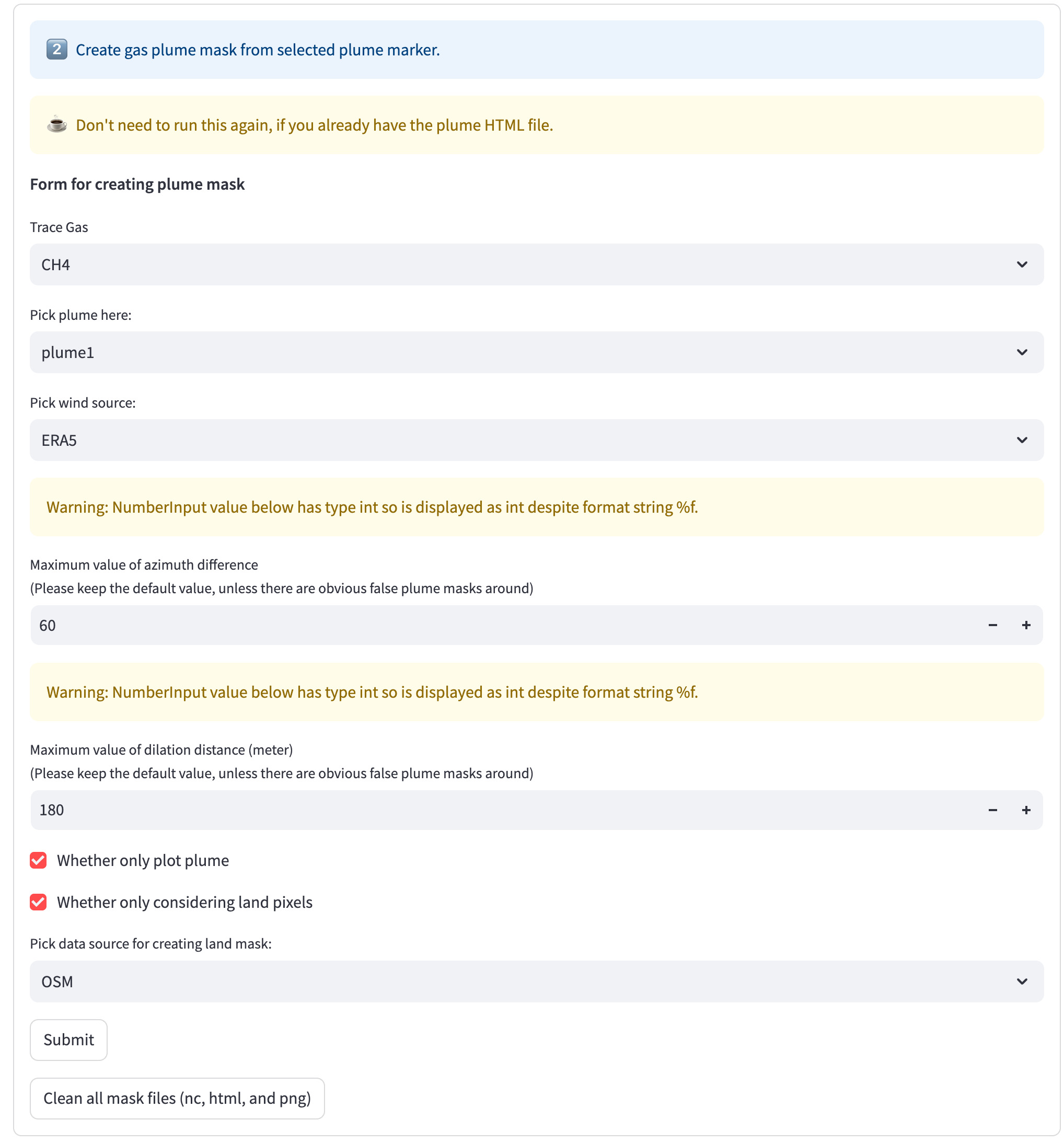
Once plume source locations are defined, select the target source and connect a priori masks. Refer to A priori mask for the definition of a priori mask. As explained in Pick plume, dilation (default: 180 m) and azimuth limits (default: 30°) are applied to coonect a priori masks.
Supported input parameters:
trace gas: The gas field to be identified.pick plume: The specific source to analyze. If multiple sources exist (e.g.,plume0,plume1), this step must be repeated for each.pick wind source: The name of wind dataset.Maximum value of azimuth difference: The maximum azimuth difference of the oriented envelope (minimum rotated rectangle).Maximum value of dilation distance (meter): The dilation distance (meter)Whether only plot plume: Plots only the plume (default: True).Whether only considering land pixels: Filters to land-only pixels (default: True)."pick data source for creating land mask: Source for land classification (default: OSM). Must match the setting inl2_process.pywhen land masking is enabled.
After configuring the parameters, submit the form.
Press the R shortcut to refresh and load the new plume HTML.
You can duplicate the browser tab to compare the mask with the full-field image on the PlumeMarker page.
If the plume mask appears incorrect, toggle “I still want to create a new plume mask” to revise settings and resubmit.
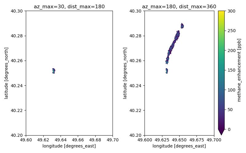
Here is an example of methane plume masks generated using different settings.
Because the default settings only include the first part of plume,
adjustments are necessary for the truncated plume.
Typically, there are usually two options: 1. increasing the azimuth difference (az_max), 2. increasing the dilation distance (dist_max).
Note
When generating land masks, three data sources are supported: “OSM”, “GSHHS”, and “Natural Earth”. OSM is used by default due to its higher resolution and accuracy. Choose carefully based on your region of interest—see Databases for more details.
Emission estimation

The emission estimation tool supports both Integrated Methane Enhancement (IME) and cross-sectional flux (CSF) methods. This module imports the same logic as described in Emission Estimation and supports the following parameters:
sitename (str): Preferred facility name. Reliable sources include: Carbon Mapper, Climate TRACE, and Global Energy Monitor.IPCC sector (str): Emission sector defined by IPCC.whether only considering land pixels: Filters calculations to land-only areas.manual wspd (float): Optional manual wind speed override (m/s).manual surface pressure (float): Optional manual surface pressure override (Pa).
Upon submission, the app will display output including emission rate estimates and associated uncertainties:
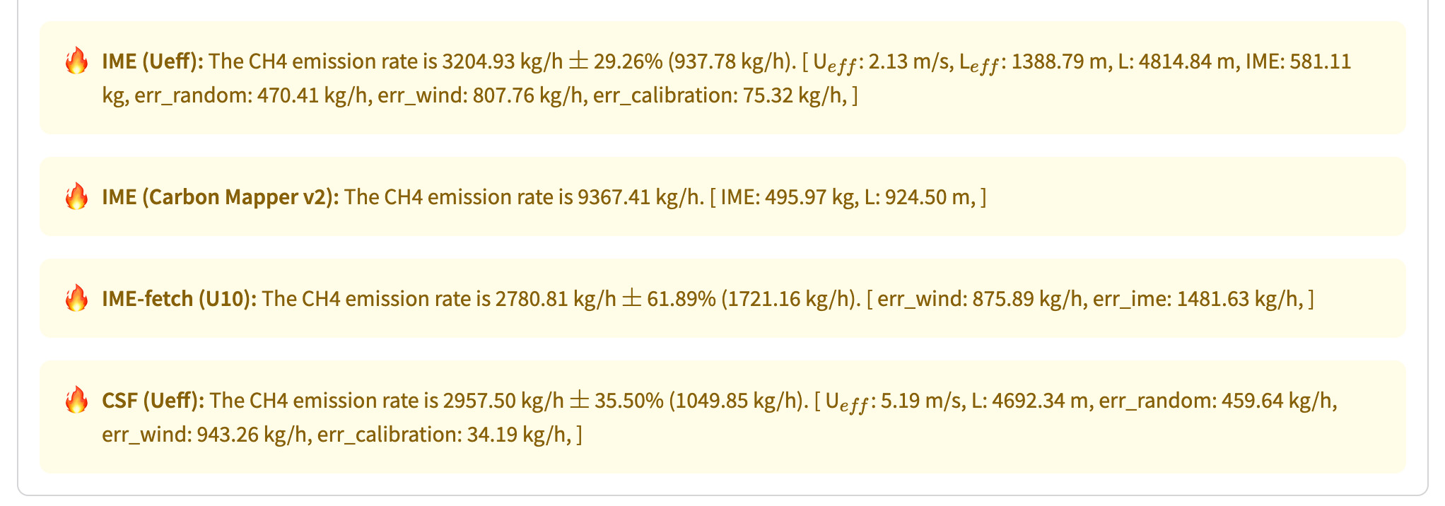
Note
It is advisable to use the IME (Ueff) and CSF (Ueff) method at this stage, as other methods are under develepment.